This page contains further notes and comments related to the topics discussed in ACCA. It is not in final form, and I expect to update it occasionally with new items.

Chapter 1

• Section 1.2: It is easy to check directly that every power series is complex analytic in its disk of convergence. Of course Theorem 1.37 proves complex analyticity of all holomorphic functions in their domain, but that proof uses Cauchy's integral formula. After an affine change of coordinate, we may assume that our power series has the form $f(z)=\sum_{n=0}^{\infty} a_n z^n$ and converges in the unit disk $\DD$. We want to show that for every $p \in \DD$ the function $f$ can be represented by a convergent power series $\sum_{n=0}^{\infty} c_n (z-p)^n$ in the disk $\DD(p,1-|p|)$. Let $z \in \DD(p,1-|p|)$ so $|z-p|=r-|p|$ for some $|p| \leq r < 1$, and write $$\begin{aligned} f(z) & = \sum_{n=0}^{\infty} a_n z^n = \sum_{n=0}^{\infty} a_n (z-p+p)^n \\ & = \sum_{n=0}^{\infty} \sum_{k=0}^n a_n {n \choose k} (z-p)^k p^{n-k} \\ & = \sum_{k=0}^{\infty} \underbrace{\left( \sum_{n=k}^{\infty} {n \choose k} a_n p^{n-k} \right)}_{c_k} (z-p)^k. \end{aligned}$$ The only caveat is to make sure that interchanging the order of summations in the above computation is legitimate. But that follows from absolute convergence of the double sum. Indeed, $$\sum_{k=0}^n {n \choose k} |z-p|^k |p|^{n-k} = \sum_{k=0}^n {n \choose k} (r-|p|)^k |p|^{n-k} = r^n,$$ so $$\sum_{n=0}^{\infty} \sum_{k=0}^n |a_n| {n \choose k} |z-p|^k |p|^{n-k} = \sum_{n=0}^{\infty} |a_n| r^n <+\infty.$$
• Section 1.3: There is a geometric interpretation of complex integration due to G. Polya which originally appeared in his complex analysis book (written jointly with G. Latta, now out of print). A lucid elementary account of this interpretation can be found in T. Needham's Visual Complex Analysis, Oxford University Press, 1997. The basic idea is to associate to a holomorphic function $f=u+iv$ the vector field $X= u \, \bd/\bd x - v \, \bd/\bd y$ (identified with the conjugate function $\bar{f}$) and to express the complex integral of $f$ along a curve in terms of the work and flux of $X$ along that curve. The connection can be used to tie in Cauchy's theorem in complex analysis with Stokes' theorem from vector calculus.
• Section 1.3: In several places (such as the proof of Theorem 1.29), path connectivity of a domain is used to join pairs of points by a curve along which some function is to be integrated. These curves can always be taken piecewise affine (polygonal) and therefore piecewise $C^1$. In fact, an easy exercise shows that if $U \subset \CC$ is open and connected and $p \in U$, then the non-empty set of $z \in U$ that can be joined to $p$ by a piecewise affine curve in $U$ is both open and closed in $U$, hence must be all of $U$.
• Section 1.5: The most basic property of order at a point for holomorphic functions is $$\ord(fg,p)=\ord(f,p)+\ord(g,p),$$ which extends to meromorphic functions (Definition 3.9) as well as infinite products (Theorem 8.15). If we define the divisor of $f \in \MM^{\ast}(U) := \MM(U) \sm \{ 0 \}$ as the element $(f) := \sum_{p \in U} \ord(f,p) \, p$ of the free Abelian group ${\mathcal G}(U)$ generated by the points of $U$, we obtain the fundamental relation $(fg) = (f)+(g)$. In other words, $f \mapsto (f)$ is a homomorphism from the multiplicative group $\MM^{\ast}(U)$ to the additive group ${\mathcal G}(U)$. Divisors provide a convenient language to express data associated with zeros and poles of meromorphic functions.

Chapter 2

• Section 2.3: Here is a beautiful application of winding numbers, following A. P. Morse, to prove Brouwer's fixed point theorem in dimension 2 according to which every continuous map $f: \ov{\DD} \to \ov{\DD}$ has a fixed point. Assume $f(p) \neq p$ for all $p \in \ov{\DD}$. Then $H: [0,1] \times [0,1] \to \Cstar$ defined by $$H(t,s) := \begin{cases} f(2s \, e^{2\pi it})- 2s \, e^{2\pi it} & \ \ s \in [0,1/2] \\ (2-2s)f(e^{2\pi it})-e^{2\pi it} & \ \ s \in [1/2,1] \end{cases}$$ is a free homotopy between the constant map $\gamma_0(t):=H(t,0)=f(0)$ and the loop $\gamma_1(t):=H(t,1)=-e^{2\pi it}$. But this leads to the absurd conclusion $$0 = \wind(\gamma_0,0) = \wind(\gamma_1,0) = 1.$$

Chapter 3

• Section 3.4: Theorem 3.34 is a special case of a general result for Riemann surfaces: The sum of the residues of every meromorphic $1$-form on a compact Riemann surface is zero. See for example O. Forster, Lectures on Riemann Surfaces, Springer, 1981, p. 80.
• Section 3.5: Click here for an animated illustration of the argument principle in Example 3.44.
• Problem 12: For an alternative approach to the "if" part, observe that every closed curve $\gamma$ in $U \sm f^{-1}(\infty)$ is null-homologous in $U$ and apply the residue theorem to conclude that $\int_{\gamma} f(z) \, dz=0$. The existence of a primitive then follows from Theorem 1.29 applied to $f$ in $U \sm f^{-1}(\infty)$.

Chapter 4

• Section 4.1: The biholomorphism $\varphi: \HH \to \DD$ constructed in Example 4.5 is of course not unique. For a geometrically obvious choice, simply consider the $90^\circ$ rotation of ${\mathbb S}^2$ around the $x_1$-axis which fixes $(\pm 1,0,0)$ and sends the eastern hemisphere $x_2 > 0$ to the southern hemisphere $x_3 < 0$. The corresponding Möbius map under the stereographic projection sends $\HH$ to $\DD$ and has the formula $$z \mapsto i \frac{z-i}{z+i}.$$ The Cayley map $\varphi$ in (4.9) has a simpler formula but its geometry is a bit more involved: it corresponds to the composition of two $90^\circ$ rotations of ${\mathbb S}^2$ around the $x_2$- and $x_1$-axes, which turns out to be a $120^\circ$ rotation about the line $x_1=x_2=-x_3$.
  
  In some applications it would be easier to use other biholomorphisms $\HH \to \DD$. For example, if we want to send a particular point $p \in \HH$ to $0$, we can use the map $$z \mapsto \frac{z-p}{z-\ov{p}}.$$ For computational purposes, this is more convenient than using, say, the Cayley map $\varphi$ followed by the disk automorphism $z \mapsto (z-\varphi(p))/(1-\ov{\varphi(p)}z)$.
• Section 4.1: Click here for remarks on the cross ratio of four concurrent lines and an application in plane geometry.
• Section 4.2: It is not hard to construct domains in $\CC$ whose conformal automorphism groups contain no Möbius map other than the identity. For example, take the slit disk $U=\DD \sm [0,1)$. By the Riemann mapping theorem (Theorem 6.1) there is a biholomorphism $\phi: \DD \to U$ and the conjugation $f \mapsto \phi^{-1} \circ f \circ \phi$ gives an isomorphism $\Aut(U) \to \Aut(\DD)$. In particular, $\Aut(U)$ is a rich group of real dimension $3$. If $f \in \Aut(U)$ is a Möbius map, it must carry $\bd U$ homeomorphically onto itself, so it must preserve the unit circle and the unit interval, keeping $0$ and $1$ fixed. But the only such Möbius map is the identity.
  
  In fact, using Schwarzian derivatives (Chapter 6, Problem 27) one can prove the following

  Theorem. Suppose $U \subsetneq \CC$ is a simply connected domain. If $\Aut(U) \subset \text{Möb}$, then $U$ is a round disk or a half-plane.

  Proof. Take a biholomorphism $\phi: \DD \to U$ given by the Riemann mapping theorem. By the assumption, $g= \phi \circ f \circ \phi^{-1}$ is Möbius for every $f \in \Aut(\DD)$. We have $S_{\phi \circ f} = S_{g \circ \phi}$, or $$S_\phi \circ f \cdot (f')^2 + S_f = S_g \circ \phi \cdot (\phi')^2 + S_\phi.$$ Since $S_f=S_g=0$, this reduces to $$S_\phi \circ f \cdot (f')^2 = S_\phi \qquad \text{for every} \ f \in \Aut(\DD).$$ In particular, choosing $f(z)=\alpha z$ with $|\alpha|=1$, we obtain $\alpha^2 S_\phi(\alpha z) = S_\phi(z)$. Thus, the function $h(z):=z^2 S_\phi(z)$ satisfies the relation $$h(\alpha z)=h(z) \qquad \text{if} \ z \in \DD \ \text{and} \ |\alpha|=1.$$ This means $h$ is constant on each circle centered at $0$, and therefore constant by the identity theorem. Since $h(0)=0$, we must have $h=0$ everywhere. It follows that $S_\phi=0$ everywhere in $\DD$, so $\phi$ is the restriction of a Möbius map. This proves $U=\phi(\DD)$ is a disk or a half-plane, as claimed.

  It is clear from the above proof that the full force of the assumption $\Aut(U) \subset \text{Möb}$ is not needed. The same proof works if we only assume that for some point $p \in U$ the stabilizer subgroup $\{ g \in \Aut(U): g(p)=p \} \cong \operatorname{SO}(2)$ consists of Möbius maps.
• Problem 4: This is a special case of the Iwasawa decomposition of semi-simple Lie groups.
• Problem 18: If we rewrite the inequality as $$|f(0)| \leq \frac{|p_1 \cdots p_n|}{r^n} M,$$ we can interpret it as an improvement of the maximum principle $|f(0)| \leq M$, similar to how the classical Schwarz lemma $|f(z)| \leq |z|$ is an improvement of $|f(z)|\leq 1$.

Chapter 6

• Section 6.2: The Jordan curves $K(\{ z: |z|=r \})$ in Example 6.4 (shown in Fig. 6.3) are indeed familiar geometric objects: they are the images of ellipses with foci $-4,0$ under the inversion $z \mapsto 1/z$. This can be easily seen from the following two observations (see Example 6.6): (i) the inverted Koebe function $\hat{K}(w)=1/K(1/w)$ and the Zhukovskii map $Z(w)=w+w^{-1}$ are related by the formula $\hat{K}=Z-2$; (ii) $Z$ maps the family of circles $|z|=r > 1$ to the family of ellipses with foci $\pm 2$.
• Section 6.2: It is fun to notice that the Zhukovskii map $Z$ has already made an appearance in the context of the Möbius group: By (4.17), $Z+2$ is the map that sends the fixed point multiplier $\alpha$ to the trace-squared invariant $\tau$.
• Section 6.2: A nice elementary account of the proof of de Branges' Theorem 6.15 can be found in J. Korevaar, Ludwig Bieberbach's conjecture and its proof by Louis de Branges, American Mathematical Monthly 93 (1986) 505 514.
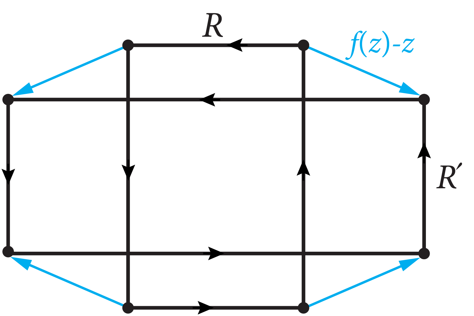• Section 6.3: The conformal invariance of the modulus of a rectangle (Example 6.31) has an unusual and ingenuous proof which I have learned from Z. He and O. Schramm's paper Koebe uniformization and circle packings, Annals of Mathematics, 137 (1993) 369-406. They formulate it in terms of indices of holomorphic vector fields but it can also be expressed in a more traditional language as follows. Take rectangles $R:=[0,a] \times [0,b]$ and $R':=[0,a'] \times [0,b']$ and consider a conformal map $f: R \to R'$ sending each corner of $R$ to the corresponding corner of $R'$. Our goal is to show that $b/a=b'/a'$. Suppose not, and say $b/a>b'/a'$. After composing $f$ with an affine map, we may arrange the position of the two rectangles as in the figure. Let $v(z)=f(z)-z$. On the one hand, the image of the positively oriented boundary $\bd R$ under $v$ has winding number $-1$ with respect to the origin. On the other hand, by the argument principle, this winding number is the number of zeros of $v$ in $R$ counting multiplicities, so it must be $\geq 0$. Contradiction!

Chapter 7

• Section 7.2: There is a simple relation between the Poisson and Cauchy integral formulas in the unit disk. The key observation is that the Poisson kernel at $z \in {\mathbb D}$ measures the difference between the values of the Cauchy kernel at $z$ and $1/\bar{z}$. In fact, if $|\zeta|=1$, then $$\begin{aligned} \frac{1}{\zeta-z} - \frac{1}{\zeta-1/\bar{z}} & = \frac{1}{\zeta-z} + \frac{\bar{z} \bar{\zeta}}{\bar{\zeta}-\bar{z}} \\ & = \frac{\bar{\zeta}(1-|z|^2)}{|\zeta-z|^2} = \frac{1}{\zeta} P(\zeta,z). \end{aligned}$$ Thus, the Poisson integral of $h \in L^1({\mathbb T})$ can be expressed as $$\begin{aligned} {\mathcal P}[h](z) & = \frac{1}{2\pi i} \int_{\mathbb T} P(\zeta,z) h(\zeta) \frac{d\zeta}{\zeta} \\ & = \frac{1}{2\pi i} \int_{\mathbb T} \frac{h(\zeta)}{\zeta-z} \, d\zeta - \frac{1}{2\pi i} \int_{\mathbb T} \frac{h(\zeta)}{\zeta-1/\bar{z}} \, d\zeta. \end{aligned}$$ If we denote the Cauchy transform of $h$ by $$H(z):= \frac{1}{2\pi i} \int_{\mathbb T} \frac{h(\zeta)}{\zeta-z} \, d\zeta,$$ which is holomorphic away from the unit circle, we obtain $${\mathcal P}[h](z)=H(z)-H(1/\bar{z}) \qquad \text{for} \ |z| < 1.$$ This represents the Poisson integral as the sum of a holomorphic and an anti-holomorphic function in the disk, and provides another proof for the fact that ${\mathcal P}[h]$ is harmonic.
• Section 7.2: The Dirichlet problem for a planar domain $U$ asks to extend a given continuous function on $\bd U$ to a harmonic function in $U$. It is a fundamental problem with a long history and central importance in applications. The Poisson integral provides a solution in the case $U=\DD$ (Corollary 7.30) which, when combined with the Riemann mapping and Carath odory theorems, leads to a solution when $U$ is simply connected with locally connected boundary. The possibility of solving the Dirichlet problem in a domain can be equivalently formulated in terms of another analytic condition often known as regularity of the domain. A useful sufficient condition for regularity of $U$ is that no connected component of $\bd U$ reduces to a point. On the other hand, any domain with an isolated boundary point is certainly non-regular, while domains such as complements of Cantor sets may or may not be regular. For a concise treatment of the Dirichlet problem, based on Perron's method, see T. Ransford's Potential Theory in the Complex Plane, Cambridge University Press, 1995.

Chapter 8

• Section 8.2: The universal choice of $d_n=n$ in Theorem 8.21 is not optimal, as much smaller choices such as $d_n= \lfloor \log n \rfloor$ still work. In fact, for any sequence $r_n \to +\infty$ and any given $r>0$ we have $r/r_n < e^{-2}$ for all large $n$, which implies $$\left( \frac{r}{r_n} \right)^{d_n+1} \leq e^{-2(\log n+1)} \leq \frac{\con}{n^2} \qquad \text{for all large} \ n.$$
• Section 8.3: For $f$ holomorphic in a neighborhood of $\overline{\mathbb D}$, the inequality $$\begin{equation}\label{jen} \log |f(0)| \leq \frac{1}{2\pi} \int_0^{2\pi} \log |f(e^{it})| \, dt \end{equation}$$ is an immediate consequence of Jensen's formula (8.8). It is stronger than the inequality $$|f(0)| \leq \frac{1}{2\pi} \int_0^{2\pi} |f(e^{it})| \, dt$$ given by Cauchy's integral formula. Here is a neat elementary proof of ($\ref{jen}$) that uses nothing more than the standard maximum principle. Take $\omega=e^{2\pi i/n}$ and for $0 \leq k \leq n-1$ let $M_k$ denote the maximum value of $|f|$ on the closed segment $I_k$ of the unit circle from $\omega^k$ to $\omega^{k+1}$. Define $g(z):=\prod_{k=0}^{n-1} f(\omega^k z)$. For any $z$ on the unit circle, the $n$ points $z, \omega z, \ldots, \omega^{n-1} z$ fall in $n$ distinct segments $I_0, I_1, \ldots, I_{n-1}$. Thus, $|g| \leq \prod_{k=0}^{n-1} M_k$ on the unit circle. The maximum principle applied to $g$ then gives $$|f(0)|^n = |g(0)| \leq \prod_{k=1}^{n} M_k,$$ or $$\log |f(0)| \leq \frac{1}{n} \sum_{k=1}^n \log M_k.$$ Letting $n \to \infty$ now gives the result.
• Section 8.3: Suppose $f: \DD \to \DD$ is holomorphic with $f(0)\neq 0$. In Example 8.33 we used Corollary 8.31 (a consequence of Jensen's formula) to prove the bound $\text{N}(r) \leq \log|f(0)|/\log r$ for the number of zeros of $f$ in the disk $\DD(0,r)$. This bound can also be obtained directly from an elementary incarnation of the Schwarz lemma as follows (compare problems 17 and 18 in Chapter 4). Let $p_1, \ldots, p_n$ denote the zeros of $f$ in the disk $\DD(0,r)$, where each zero is repeated as many times as its order. The finite Blaschke product $B(z):=\prod_{k=1}^n (z-p_k)/(1-\ov{p_k}z)$ has the same zeros of the same orders as $f$, so the ratio $g:=f/B$ extends to a holomorphic function in $\DD$. Since $|g(z)| \leq 1/|B(z)|$ and $|B(z)| \to 1$ as $|z| \to 1$, the maximum principle shows that $|g| \leq 1$ or $|f| \leq |B|$ everywhere in $\DD$. In particular, $|f(0)| \leq |B(0)|=|p_1 \cdots p_n| \leq r^n$, or $n \leq \log|f(0)|/\log r$.

Chapter 9

• Sections 9.1 and 9.2: In general, sums over countably inifnite sets such as the integers $\ZZ$ or lattices $\Lambda \subset \CC$ do not make sense unless some order on the set (i.e., a bijection with natural numbers $\NN$) is specified. This issue is altogether ignored in the examples $\sum_{n \in \ZZ}$ or $\sum_{\omega \in \Lambda}$ that occur in these sections because in all such instances the sum (in some order) is absolutely convergent, so it has a well-defined value independent of the order of summation.

Chapter 10

• Section 10.1: A power series may well diverge at regular points of its circle of convergence. A basic example is $\sum_{n=0}^{\infty} z^n$ which diverges everywhere on $\TT$ even though every point of $\TT \sm \{ 1 \}$ is regular. However, the following result (due to Fatou) holds: Let $f(z)=\sum_{n=0}^{\infty} a_n z^n$ have radius of convergence $1$ and assume $\lim_{n \to \infty} a_n=0$. If $q \in \TT$ is a regular point of $f$, then $\sum_{n=0}^{\infty} a_n q^n$ converges. See for example, S. Saks and A. Zygmund, Analytic Functions, 3rd ed., Elsevier, 1971, pp. 245-246.
• Section 10.1: The sharpest version of Hadamard's gap theorem (Theorem 10.9) was proved in 1899 by E. Fabry: If $f(z)=\sum_{n=0}^{\infty} a_n z^{m_n}$ has radius of convergence $1$, where $m_n/n \to +\infty$, then $\TT$ is the natural boundary of $f$. Fabry's result is in a sense optimal since in 1942 G. Polya showed that if $\liminf_{n \to \infty} m_n/n < +\infty$, there is a power series of the form $\sum_{n=0}^{\infty} a_n z^{m_n}$ with radius of convergence $1$ for which $\TT$ is not the natural boundary.
  
  The classical example which is covered by Fabry's gap theorem (but not by Hadamard's) is the theta series $\theta(z)=1+2\sum_{n=1}^\infty z^{n^2}$ that occurs in number theory.
• Section 10.1: In the spirit of the results of this section, let us mention the following remarkable theorem of Jentzsch: If the power series $\sum_{n=0}^\infty a_n \, z^n$ has radius of convergence $0 < R < +\infty$, every point of the circle $|z|=R$ is an accumulation point of the zeros of the sequence of partial sums $s_n(z)=\sum_{k=0}^n a_k \, z^k$. (Basic example: $\sum_{n=0}^\infty z^n$ for which $s_n(z)=(1-z^{n+1})/(1-z)$ and every point of the circle $|z|=1$ is accumulated by a sequence of roots of unity.) See E. Titchmarsh, The Theory of Functions, Oxford University Press, 2nd ed., 1939, pp. 238-241.

Chapter 12

• Section 12.2: In 1907 A. Denjoy conjectured that every transcendental entire function of growth order $\rho$ has at most $2\rho$ (finite) asymptotic values. After important partial results by T. Carleman, the full conjecture was finally proved by Ahlfors in 1929.
• Section 12.3: Given any collection of not necessarily distinct points $c_1, \ldots, c_{d-1} \in \DD$ there is a proper holomorphic map $f:\DD \to \DD$ (i.e., a finite Blaschke product) of degree $d$ whose critical points are the $c_k$. Moreover, $f$ is uniquely determined up to postcomposition with an element of $\Aut(\DD)$. See S. Zakeri, On critical points of proper holomorphic maps on the unit disk, Bull. London Math. Soc. 30 (1998) 62-66, and compare the additional problems of Chapter 12.
  
  The corresponding question for the other two simply connected domain types, the complex plane and the Riemann sphere, have trivial and surprising answers. Every proper holomorphic map $\CC \to \CC$ is a polynomial, and it is easy to see that any $d-1$ points in the plane can be realized as the critical points of a polynomial of degree $d$, which is unique up to post-composition with an element of $\Aut(\CC)$. In the case of the Riemann sphere, however, both the existence and uniqueness parts of this statement are false. Every proper holomorphic map $\Chat \to \Chat$ of degree $d$ is a rational map with $2d-2$ critical points counting multiplicities. There are certainly configurations of points on the sphere which cannot be realized as the critical set of a rational map. For example, it is impossible to realize a single point of multiplicity $2$ as the critical set of a rational map, since any such map would have degree $2$ and local degree $3$ near the double critical point. On the other hand, any collection of $2d-2$ distinct points on the sphere can be realized as the critical set of a rational map of degree $d$, but typically there is more than one way to get such a map, even up to postcomposition with an element of $\Aut(\Chat)$. See L. Goldberg, Catalan numbers and branched coverings by the Riemann sphere, Advances in Math. 85 (1991) 129 144.
• Section 12.4: Our treatment of holomorphic branched coverings is restricted to spherical domains, but the natural framework of the theory is proper holomorphic maps between Riemann surfaces. In particular, every non-constant holomorphic map between compact Riemann surfaces is automatically a finite-degree branched covering and the analog of the Riemann-Hurwitz formula holds (where the Euler characteristic is related to genus by $\chi=2-2g$). An instructive example is the Weierstrass $\wp$-function of a lattice $\Lambda \subset \CC$ (see section 9.2) which induces a non-constant holomorphic map $\wp: \CC / \Lambda \to \Chat$ of degree $d=2$. According to the Riemann-Hurwitz formula, this function has $2\chi(\Chat)-\chi(\CC / \Lambda)=4$ critical points counting multiplicities, consistent with our elementary analysis in Theorem 9.11.

Chapter 13

• Section 13.1: The modular group $\Gamma \cong \PSL_2(\ZZ)$ is isomorphic to the free product $(\ZZ/2\ZZ) \ast (\ZZ/3\ZZ)$. In fact, Lemma 13.10 shows that the two elements $A(z)=z+1$ and $B(z)=-1/z$ generate $\Gamma$, and it can be verified that $\Gamma$ has the presentation $\langle A,B: B^2=(AB)^3=I \rangle$. This amounts to showing that each element of $\Gamma$ can be written uniquely as a reduced word in $B$ and $C=AB$. A short, beautiful proof of this fact can be found in R. Alperin, $\PSL_2(\ZZ) = \ZZ_2 * \ZZ_3$, American Mathematical Monthly 100 (1993) 385 386.